
What Can You Do about a Lousy Forecast?
By Quentin Samelson, Sr. Managing Consultant, Global Business Services at IBM

One of the oldest jokes in operations management is that “accurate forecast” is an oxymoron. But it seems that many companies have gotten so used to poor forecast quality that they’ve lost focus on this business-critical issue. Improving forecast accuracy by even a small amount can have a massive, and very positive effect on company performance – lowering inventory, improving profits, reducing excess & obsolescence, and improving customer satisfaction.
Understanding forecast (in)accuracy is really about understanding customer behavior, and the kind of markets where most companies operate. There are all sorts of reasons that customer demand can be difficult to predict:
- Actual consumer demand can be influenced by many external elements – the economy, the number of options available to the purchaser, the weather, advertising and social media, even the behavior of other companies.
- At their core, consumer purchase decisions are almost always optional. There aren’t many items in life that people have to buy; and even in those cases, people (and companies) usually have the choice of several or even hundreds of options.
- Although the demand for most products ultimately is affected by consumer behavior, your company’s products may be targeted at other companies (or governments). In that case, demand for your product can be influenced by companies’ own strategies and constraints, as well as by regulations, politics, and other factors like cash flow, inventory, availability of resources, etc.
- Whether you make a consumer or an industrial product, most companies sell to other companies, and the purchasing people at those companies (a) may not have good command of their own customers’ demand; and (b) may utilize their demand forecast as a negotiating tool. (Sometimes a buyer will hold back demand until the end of a quarter in hopes of a discount; sometimes a buyer will over-forecast to “lock up” supply.)
So what is a demand planner supposed to do? There are some really impressive statistical and cognitive tools[1] that have become available in the last few years that can make a substantial difference in forecast accuracy for individual SKUs (Stock Keeping Units) and businesses; we’ll talk about those in a future post. Before you invest in the latest tools, it’s important to first gain an understanding of what your demand data means, where it matters, and which SKUs will be worth an investment to reduce forecast error.
Three steps will help you (a) discover whether any simple changes can remove errors from your forecast; (b) identify how demand data impacts your company’s production and procurement plan; and (c) identify which SKUs really need forecast accuracy improvement, and which can be managed with existing methods.
I. Understand what the demand data means.
If you receive a demand forecast from customer A like the one above, and an identical one from customer B, do they mean the same thing? Not necessarily. Company A may be forecasting “1000 pieces of product NX-5895 for delivery during the week ending 20. April.” Company B may be forecasting “1000 pieces of product NX-5895 to ship on 20. April.” That seems like a minor difference, but the fact is that you would need to have 1000 pieces ready to ship to Company A a week earlier than for Company B. There are a number of variations on this; your contract with Company B may require you to be able to ship up to 15% over their forecast, for instance.
Just because the data looks the same, doesn’t mean it is the same. Understanding this can provide you with a much better understanding of what your customer’s forecast really means.
II. Understand your organization’s supply planning methods and concerns.
If you need to ship 1000 pieces of product NX-5895 on April 20th, will you just pull 1000 pieces from stock on that day, or do you need to build them? When would you need to start them, and how many do you need to start in order to be confident of getting 1000 pieces that meet the customer’s requirements?
When do you need the components to arrive in order to build 1000 pieces? And, understanding the lead times of those components, when do you need to order the components? This is an enormous subject by itself, but your demand planning will be better if you understand how it is used to create a supply plan.
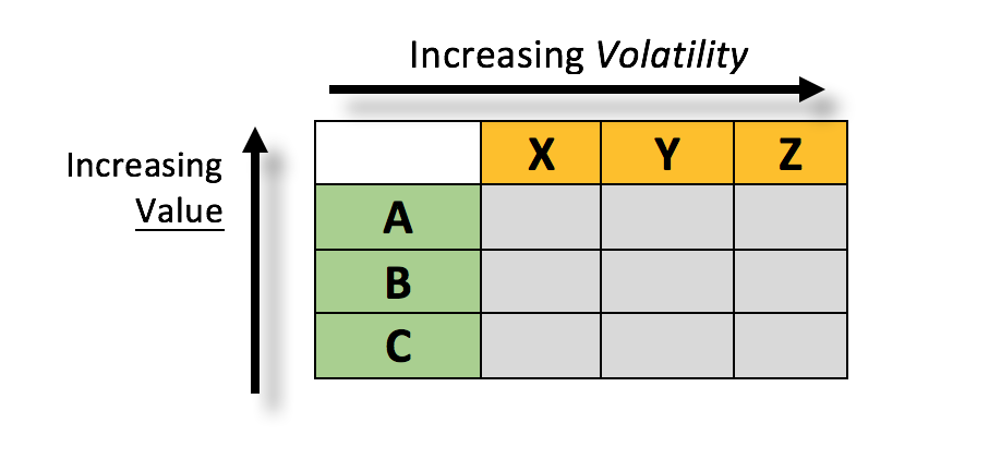
III. Understand your SKUs’ variability vs. value
Most of us are familiar with Pareto’s principle applied to purchase value (ABC codes), but the concept becomes much more powerful if combined with a similar analysis of SKU demand variability. The goal is to identify SKUs according to the variability of their demand[2]:
• X = very little variation. Future demand is relatively steady and can be reliably forecasted.
• Y = some variation. Future demand isn’t steady, but some (at least) of the variation can be predicted (due to seasonality, economic factors, etc.). Forecasts are not as reliable but are still useful.
• Z = the most variation. Demand can fluctuate strongly or be very sporadic. Reliable forecasting is nearly impossible.
To categorize items into X, Y, and Z classifications, a typical process is to calculate the normalized demand volatility for each SKU. (Normalizing just means dividing the standard deviation of demand by the average demand for the item, so you can compare a product with high demand to a product with lower demand.) You would use an equation like this:
XYZ value = (std deviation of demand) / (average demand)
Then sort in increasing XYZ value, and identify where to draw the lines between X and Y, then Y and Z. (You can simply assign the first 20% of the SKUs to X, the next 30% of SKUs to Y, and the remainder to Z; but longer-term you should try to associate a set of XYZ value ranges with relative stability (X), or relative volatility (Z) at your company, with Y in between.[3]
The goal is to be able to build a table like the one below. The table shows that your company can develop a specific supply strategy for each combination (AX, for instance, is far easier to manage than BZ).
More important for the demand planning function: understanding how many, and which, SKUs fall into the difficult categories like AZ will help you get ready for the next stage of the process: applying statistical and cognitive tools to reduce forecast errors. There may be no need to worry about reducing forecast error for the SKUs in the “X” category, but the AY and AZ categories will be critical. Understanding where the biggest opportunities lie is critical. If you have a large number of “A” SKUs that fall into the “Z” XYZ category, focusing your attention on those products can produce a much greater impact than if your forecast improvement efforts are unfocused.
[1] As a teaser, take a look at these links: https://www.ibm.com/blogs/insights-on-business/electronics/demand-forecasting-reinvented/
http://www.ibmbigdatahub.com/blog/predictive-forecasting-cognitive-erahttps://scholarspace.manoa.hawaii.edu/bitstream/10125/41281/1/paper0132.pdf
[2] Further explanation of this concept, with some helpful graphics, can be found at https://www.cgma.org/resources/tools/cost-transformation-model/xyz-inventory-management.html
[3] This may be the trickiest part of the process, but it should improve over time. Some companies have used an alternative calculation for the XYZ value, to obtain a somewhat more predictable range of values. The alternative calculation is XYZ value = [(std deviation of demand)/(average demand)] x [(range of demand)/(average demand)]